2008-09-22

Python inside LaTeX (and Sage too)

I discovered recently, that it is possible to run Python scripts from LaTeX documents and use the to generate document's content. This can be used to read/convert data, generate tables and figures, do on-the-fly calculations.

How to run Python code from LaTeX:

  • download python.sty. Put it in the same directory as the LaTeX document
  • \usepackage{python}
  • Put Python code inside \begin{python}\end{python} environment. Whatever this code prints, will become part of the LaTeX document.
  • Run LaTeX with -shell-escape option (this permits running external code from LaTeX)
This is an example of the LaTeX document and the PDF produced.

And some more advanced examples are in this LaTeX file (see also the PDF). They cover symbolic calculations from inside LaTeX, plotting and variable persistence between python environments.

P.S. What's more, one can even embed the full-featured symbolic math package Sage into LaTeX. For this purpose use sagetex package. By the way, you do not need to install Sage to start using it, please check out its web-version. It is really powerful.

Links:

This post in Russian: Python внутри LaTeX (и математический пакет Sage тоже)

Visualizing altitude and velocity profiles of GPS tracks

I think that altitude and velocity profiles of GPS tracks is one of the most intereseting forms of their representation. One can use gpsvisualizer.com to plot such profiles. However, I prefer having free tools for such a simple thing.

Here I offer my own python script gpxplot, which extracts profile data from a GPX file and plots a profile. This is a direct link: gpxplot.py.

There are two important features of the script:

1) GPX file may consist of two or more separate tracks. Each track may consist of several disconnected segments. The script preserves this segmentation of the track.

2) GPX files do not contain explicit information about distane travelled. The script calculcates it using haversine formula (as if the Earth were spherical).

The script can either output profile data in a convinient tabular form, or generate a gnuplot script and call gnuplot to do actual plotting.

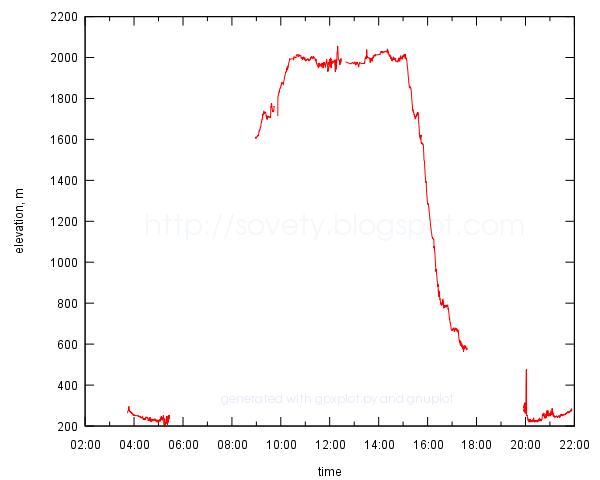
Usage examples are given on a Google Code page. This is what a result may look like:
example of a time-altitude profile plotted to SVG file with gnuplot

Update: Now there is also online version of the script. Just upload a track and embed the plot in whatever page you want.

Links:

This announcement in Russian: Визуализация профилей высоты и скорости GPS-треков

2008-07-15

Auto-building LaTeX documents with SCons

How many commands does it take to compile LaTeX document?
1. pdflatex mypaper.tex
2. bibtex mypaper
3. pdflatex mypaper.tex
4. pdflatex mypaper.tex
— and how many times do you have to type them when you edit an article? A lot.

Fortunately, there is a simple cure. A SCons build system. Install it and create a new SConstruct file where the LaTeX document lives, with a contents like this:

PDF(target = 'mypaper.pdf', source = 'mypaper.tex')
Then just run
$ scons
And SCons will automatically run bibtex if you use it, it will run PDFLaTeX as many times as it needs (SCons is smart enough to read the log file of the LaTeX), SCons will remember MD5 sum of the source file and will avoid re-compiling the PDF if the source file did not change. Very convenient!

I also prefer to re-build the PDF whenever I change any of the figures. Given that my figures are in imgs/ subfolder and all are either *.pdf or *.png files, I can create a list of “source” files using SCons' Glob function. This is what SContstruct then looks like:

src_list = [ 'mypaper.tex', Glob('imgs/*.pdf'), Glob('imgs/*.png') ]
PDF(target = 'mypaper.pdf', source = src_list)
Of cource, one can still use make to compile LaTeX documents. This is a good Makefile for a start.

This post in Russian: Автоматическая компиляция документов LaTeX

2008-06-09

antiodt: view OpenOffice documents as plain text

I don't like launching heavy office applications just to read a file. And there are antiword and wv to read MSWord *.doc files, unrtf to read RTF, and pdftotext to read PDF. Only open, ISO standard, ODT (OpenDocument, produced by OpenOffice) cannot be read that way. o3read seems to be useless for the new ODT files.

So, this is a one-and-half-line script I use to view OpenOffice files quickly from the shell prompt (antiodt):

#!/bin/sh
unzip -p "$1" content.xml | \
xmlstarlet sel -N text="urn:oasis:names:tc:opendocument:xmlns:text:1.0" \
  -T -t -m '//text:p' -v . -n | less
Any ODT is just a normal ZIP archive with an XML file with all the contents. I used xmlstarlet to extract text paragraphs from that XML. Certainly, all formatting is lost, but it is fast.:
$ antiodt document.odt
I got an idea from here.

Update 2009-09-23: To convert ODT to plain text and preserve some formatting, use odt2txt.py script. It converts ODT to Markdown.

This post in Russian: antiodt: просмотр документов OpenOffice в виде простого текста

2008-04-15

Various LaTeX tips

I decided to bring together LaTeX tips from my other blog.

How to change line spacing?

To change spacing between baselines:
% to set one-and-half spacing
% put before \begin{document}
\renewcommand{\baselinestretch}{1.5}
More flexible way is provided by setspace package. It allows to change line spacing for parts of the text. To use the package, add before \begin{document}:
\usepackage{setspace}
\onehalfspacing % one-and-half spacing globally
% or \singlespacing % normal spacing
% or \doublespacing % double spacing
% or \setstretch{factor} % arbitrary spacing
Then after \begin{document} you can use onehalfspace and doublespace environments:
\begin{onehalfspace}
This text will be set with one-and-half line spacing.
\end{onehalfspace}
\begin{doublespace}
This text will be set with double line spacing.
\end{doublespace}

How to change margins?

The easiest way is to use geometry package, add before \begin{document}:
\usepackage[left=2cm,right=2cm,top=2cm,bottom=2cm,bindingoffset=0cm]{geometry}
To change layout and margins of the particular pages use chngpage package.

How to fit the text on one page?

First, try to \enlargethispage:
\enlargethispage{2\baselineskip} % add two more lines to this page
\pagebreak % finish the page
If you want to shrink the text, use the “starred” version \enlargethispage*{length}:
\enlargethispage*{\baselineskip}

How to rotate a page?

Use lscape package and the landscape environment it provides to rotate arbitrary pages. This may be useful to fit wide tables or figures:
% before \begin{document}
\usepackage{lscape}
% after \begin{document}
...
\begin{landscape}
...
This text will appear on a rotated, i.e. landscape, page.
...
\end{landscape}

Why figure numbering is wrong?

Check your figure environment. \label should always go after \caption. \caption first, \label second. The right template for the figure is:
\begin{figure}
... % insert your figure here
\caption{Caption text}
\label{fig:myfigure}
\end{figure}
See also figure numbers wrong in LaTeX.

How to make my own BibTeX style?

Fortunately, it is easy. Use makebst.tex program. In my system I can run it as
$ latex /usr/share/texmf-texlive/tex/latex/custom-bib/makebst.tex
Choose merlin as a template, choose any name for your style (e.g. mystyle), answer all the questions patiently. Finally, copy ile mystyle.bst to the directory with your article. Use it like this:
\bibliographystyle{mystyle}
\bibliography{bibfile}

How to enable/disable page numbering?

To disable page numbers:
\pagestyle{empty} % no page numbers
To enable page numbers:
\pagestyle{plain} % enable page numbers
To change it just for one page:
\thispagestyle{style}
To do more fancy things, use fancyhdr package.

How to make the PDF I produce with PDFLaTeX searchable?

Answer:
\usepackage{cmap}

How to strike-through or highlight the text?

To strike through words in LaTeX use package ulem:
% before \begin{document}:
\usepackage{ulem}
…
% in the text, after \begin{document}:
\sout{Wrong.} Right.
The result will be something like this:
Wrong. Right
To highlight words with different colour, use xcolor package:
% before \begin{document}
\usepackage{xcolor}
…
% after \begin{document}
I want some words to \textcolor{red}{stand out}.
Expect the result to be:
I want some words to be stand out.
If you want to change the background colour, \colorbox will help you:
% to make text appear on whitish blue (blue 50% – white 50%)
\colorbox{blue!50!white}{Text on whitish blue background}
And the result:
Text on whitish blue background

How to make notes on margins?

This is what \marginpar command does:
\marginpar{This text appears in the margin.}
Check also Todo notes in LaTeX by Henrik Skov Midtiby. He uses \marginpar to add side notes to the draft document. They look awesome (but don't work for me). I settled on a simplified version. Put before \begin{document}:
%%% todo notes, idea from
%%% http://midtiby.blogspot.com/2007/09/todo-notes-in-latex.html
%%%
\newcommand{\todo}[1]{
      \addcontentsline{tdo}{todo}{\protect{#1}}
      \colorbox{orange!90!black}{\textcolor{white}{\tt TODO}}
      \marginpar{\colorbox{orange!90!black}{\textcolor{white}{
      \parbox{4cm}{\small\tt\raggedright TODO:\\#1}
      }}}
}
\makeatletter
\newcommand\listoftodos{\clearpage\section*{Todo list} \@starttoc{tdo}}
\newcommand\l@todo[2] {\par\noindent {\Large $\Box$\;#1\dotfill\makebox[1.5em][r]{#2}\;}\par}
\makeatother
Then in the text add notes with:
\todo{rewrite this}
and finally add in the end:
\listoftodos
2008-02-05

Effective conversion from raster to EPS

There are several ways to use raster images (JPEG, PNG, TIFF) in LaTeX. Fortunately, PDFLaTeX supports JPEG and PNG directly. However, sometimes one has to use only EPS (PostScript) images. This post tells how to “vectorize” the raster effectively.

Out of the several conversion tools (ImageMagick, GIMP), the most effective, IMO, is sam2p. It produces the smallest EPS possible. sam2p is available in Debian repositories.

sam2p is a command line tool. To convert a PNG file image.png to EPS file image.eps do:

$ sam2p image.png EPS: image.eps

I have tried converting some Google Earth screenshots (they are fairly complicated images with a lot of details). These are the sizes of original PNG and of converted EPS images (with ImageMagick's convert and with sam2p):

$ ls -rSsk1 google-earth-screenshot*
1756 google-earth-screenshot.png
3016 google-earth-screenshot-(sam2p).eps
4304 google-earth-screenshot-(convert).eps
Certainly, sam2p-produced EPS is larger than PNG, but it is much smaller than convert-produced EPS. On some images the difference may be even bigger.

BTW, EPS produced by sam2p is EPSF-3.0, and should be compatible with the most of vector graphics software. It seems like often using sam2p may be a better option than using built-in import raster tool. At least when the size of the file matters.

Another tool for effective conversion from raster to EPS is bmeps, but I have not tried it.

P.S. I wrote this post also in Russian: Эффективная конвертация растра в EPS или PDF.

How to parse RSS 2.0 in bash

It is quite easy to use information from RSS feeds in bash scripts. I use xmlstarlet to work with XML in the shell. For example, to print the latest titles and links from my RSS feed, I can do:
RSS_URL=http://feeds.feedburner.com/usefreetools
wget ${RSS_URL} -O - 2>/dev/null | \
xmlstarlet sel -t -m "/rss/channel/item" \
  -v "guid" -n -v "pubDate" -n -v "title" -n -v "link" -n -n
Alternatively, I can use curl -g ${RSS_URL} -s instead of wget. I could have added -v "description" to see the contents of my posts.

2008-01-15

Try Exposure Blend plugin for GIMP to fake HDR

Digital cameras have relatively narrow dynamic range with respect to human eye, i.e. the difference between the brightest and the darkest grades of light the camera may capture in one shot is limited. This is the reason why some stunning scenes become badly exposed photos (with absolutely black and white areas).

There is a technique to overcome this techinical limitation of modern cameras, known as High dynamic range imaging (HDR). This technique is based on taking several pictures of exactly the same scene with different exposure levels. Then the amount of light per pixel is calculated based on all images. Finally, a combined image is produced, where information about dark areas is taken from the brigher images, and information about brighter areas is taken from the darker images. These combined images often look very good.

In GNU/Linux there is a number of Free tools which support this technique. In particular, I want to mention Cinepaint (HDR in Cinepaint tutorial) and Qtpfsgui (HDR in Qtpfsgui manual).

You just need a camera bracketing support and a tripod to start making HDR images.

However, most modern consumer-level cameras take at most 3 shots in bracketing mode, and exposure step between the shots is often limited to ±2 EV or even ±1 EV (like in my camera), which allows only slightly extend the camera's dynamic range using HDR technique.

In this case it is often easier and faster combine those three images taken with a camera using Exposure Blend plugin for GIMP (the site seems to be temporarily down, in Debian Exposure Blend plugin is part of the gimp-plugin-registry package). This is not a true HDR, but it allows to take dark details from the brighter image, and bright details from the darker image. The result is good enough, because even true HDR based on three images shot with a consumer-level camera with ±1 EV bracketing wont look much better.

In GIMP you may run the plugin from menu Xtns / Photo / Exposure Blend. Give the filenames of the three files you want to merge. All the other settings are likely OK by default.

You may get better results if your camera supports bigger bracketing step. Unfortunately, my camera does only ±1EV, which is not enough.

So I have taken a slightly different approach in the next example. I shot one image in RAW format (12 bit per color channel), and then post-processed it with UFRaw, producing three images with 0±2EV exposure correction.

Now see the results:

candle normal + candle dark + candle bright = candle blended

Just compare the original image to the composite image obtained after exposure blending (below):

Compare normal shot (above) with Exposure Blended composite image (below)

In exposure blended image the dark details are more distinct than in the original image: compare the background, the balls, the suface. Still in the bright areas there are also more details too: compare the wax of the candle. And this is with just few clicks!

I did not correct gamma, color or curves on purpose. One of the key advantages of exposure blending over HDR is that unlike in HDR in exposure blending the tone and the colors are preserved. No need to tweak tone mapping parameters. Exposure blended images always look natural.

Take a look at other Exposure Blended photos at Flickr:

Exposure Blend example 3 Exposure Blend example 4 Exposure Blend example 1 Exposure Blend example 5 Exposure Blend example 6 Exposure Blend example 2 and other photos tagged as exposureblend

P.S. I have wrote this post also in Russia, see Плагин для GIMP Exposure Blend вместо HDR

2008-01-14

About this blog

This blog is an English-speaking brother of my Russian blog about using Free (libre) software. I am going to post some tips about using GNU/Linux and other free software. I am particularly interested in graphics tools, LaTeX, visualization and numerical software, command line (shell) tricks, and general productivity with Free/Open Source software.